Introduction to Descriptive Statistics
1. Know the two basic kinds of populations: Quantitative and Qualitative.
A quantitative population characteristics is one that can be expressed numerically, such as weight, height, price and salary.
A qualitative population characteristics is one that is non-numerical, such as sex (male and female), race (Black, Hispanic, White, Asian, etc.), college major (education, math, history, communications, etc.),
2. Know the distinction between the two kinds of population observations.
The particular observation of qualitative characteristics is refer to as an attribute.
Example: The characteristic of the qualitative characteristic, marital status, may have as its attributes: single, married, divorced, or widowed.
The particular observation of quantitative characteristics is refer to as a variable (variate).
Example: Income level (a quantitative variable) can have numerical values or variate like: $25,500, $45,000, or $102,800.
Not all users of descriptive statistics use these quantities properly, so be aware of interchangeable usage of these terms. Often the term variable is used to refer to both qualitative and quantitative characteristics.
3. Know the meaning of the 4 types of quantitative
data.
Nominal data is when numbers are used to represent categories
or attributes and have no quantitative significance or meaning. Such values
often occurs when information is coded using numerical labels for data
processing.
Example: A university might designate majors by numbers, so that 5 might represent accounting students, 37 finance, 51 marketing and so on. Such data should not be treated as numerical, since relative size or value have no meaning.
Ordinal data is when values given to observations are ranked by importance, strength, or severity. The order of the data from high to low is significant, but the difference between the values have no meaning.
Example: At a company, A Senior staff is given a code of 10, a Advisory a code of 8 and a Junior staff a code of 5. Though a code of 10 denote more responsibility and pay, the difference between Senior and Advisory, 10 - 8 = 6 is meaningless.
Interval Scale is when the values given to observations reflect true differences between the values and arithmetic operation can be done with the values.
Example: The same amount of heat is required to heat the same quantity of water from an interval scale of temperature in degrees F from 40 to 60 (60-40=20) and 50 to 70 (70-50=20).
Ratio Data is data that allow for all basic arithmetic operations, including division and multiplication.
Example: Typical business data, such as revenue, cost, profit and physical measurements and time increments to name a few.
Problem: For each of the following quantities, indicate appropriate
data type according to the following classifications: (1) nominal, (2)
ordinal, (3) Interval, or (4) ratio. Answer
key
| (a) Movie ratings, 1 to 10 | (e) Employee payroll code number |
| (b) Height of men | (f) Richter scale for earthquake intensity |
| (c) Daily high temperature | (g) Task completion times |
| (d) Football player jersey numbers | (h) GMAT test scores |
4. Know the meaning and recognize examples of independent and dependent variables.
An independent variable is one that is used to determine an effect (the source or causality quantity). Often these variables are either controlled by the researcher or experimenter, or manipulated, or used to classify data.
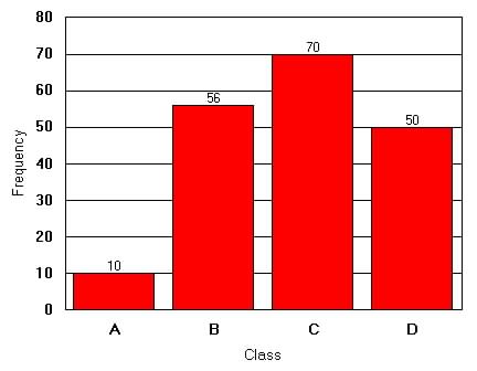
The independent variable is denoted by the symbol, X or x and represents the variable that is plotted along the x-axis or horizontal axis. (see Class in Figure 2.1)
Examples: Age (independent): Use of age to estimate average height
Humidity (independent): Use of humidity to predict chance of rain.
Test Scores: (Independent): Use of test scores to tell college potentials.
A dependent variable is the variable that measures the effects of the independent variable. Often its value is dependent on the value of the independent variable.
The dependent variable is denoted by the symbol, Y or y and represents the variable that is plotted along the y-axis or vertical axis. (see Frequency in Figure 2.1)
Example: Average Freshman College GPA( dependent): Freshman College
GPA are linked to or dependent on or related to high school Sat scores.
So college administrators might used SAT scores to determine those candidates
for admission who might do well in their first year of college (based on
GPA scores). So SAT (independent) is used to make inference about Freshman
GPA (dependent ).
| Independent Variable
(Input or X) => Cause |
Operation or Experiment
(Function or Model) |
Dependent Variable
(Output, Y) => Effect |
5. Know the meaning and recognize examples of continuous, discrete, and discrete approximations to continuous numbers.
A discrete number can only exist at specific points on a scale such as days of the week, it can only be {1, 2, 3, 4, 5, 6, 7}.
On a discrete scale there are numbers than does not exist, example, days of the week cannot be 5.5.
A continuous number may have any possible values of a number, such as whole number or fractional parts, an example is number of seconds after the start of a race, 12.5635.. seconds.
On a continuous scale any values between the extremes of the scale can exists.
A discrete approximation of a continuous value is a single number that is an approximation of a continuous measurements that is exact only in concept or principle. Example, the exact time that the first rocket was launched from earth at NASA, was an approximate time in year, month, day, hour, minutes, seconds, millisecond, etc.
On a continuous scale often it is difficult to measure precisely the true value of a point along the scale. This estimate is called the discrete approximation to the continuous. If I say that you were born in 1962, I am approximating the exact time in years, day of the year, hour, and second which in term is an approximation of a more exact time.
1. Know the fundamentals of frequency distributions.
Raw data is data that is not usually summarized or organized in any meaningful way. Often it is data as it is collected or recorded without any particular order except time of observation or sequence of observation.
Class intervals are one way of categorizing raw data according to numerical constant intervals.
Frequency is the numerical count of data in each class interval.
Sample Frequency Distribution is a representation of data showing there frequency in all class intervals.
Table 2.1 below shows the grouping of data into certain class
intervals and the frequency of each class interval. Figure 3.1 Shows
a a graphical representation of the same.
Table
2.1 Sample Frequency Distribution Table
|
Figure
2.1 Frequency Distribution Graph
|
2. Know how to determine the number of class intervals and the size of the class width for constructing frequency distributions.
The first step in contracting a frequency distribution is to:
(1) Specify the number of class interval (between 5 and 20)
(2) Determine its class width (class interval)
Figure 2.1 above has 4 class intervals (A, B, C, and D) and a class width of 10 (11 to 20 includes: 11, 12, 13, 14, 15, 16, 17, 18, 19, 20 a count of 10).
When all intervals are to be of the same width, the following rule apply:
![]()
Answer key
(a) ordinal (b) ratio (c) interval or ratio (d) nominal (e) nominal (f)
ordinal (g) ratio (h) interval