Linear correlation coefficient is a statistical parameter, r used to define the strength and nature of the linear relationship between
two variables or characteristics or attribute or quantity. In advance statistical applications the correlation coefficient may also be 
used to define non-linear, more than two variables, but in this course we concern ourselves with just comparing the relationship 
between only two variables.

The symbol for the sample correlation coefficient is r. The symbol for the population correlation coefficient is  (Greek letter rho).

The correlation coefficient presented in this text is the Person's product moment correlation coefficient (PPMC), 
named after statistician Karl Pearson, who pioneered the research in this area.
 

1. Know the meaning of the terms correlation and linear correlation.

A correlation is when two or more variables are related in some way.

Correlation requires that pairs of points be available for each set of values of each variable.

Often in the case of two variables one may arbitrarily labeled each variable X and Y.

Often the X variable represents the input variable or independent variable, that is, the variable being used to predict the 
other variable. Y often represents the output variable or the dependent variable and it is the variable being predicted.

A linear correlation is when two are more variables are related linearly, i.e. A scattered plot of the data would tend to cluster
around a straight non horizontal line. Figure 3.1 shows a scattered plot of two linearly correlated variables.
 

Figure 3.1

2. Know the meaning of high, moderate, low, positive, and negative correlation, and be able to recognize each from 
a graphs or verbal description of data.

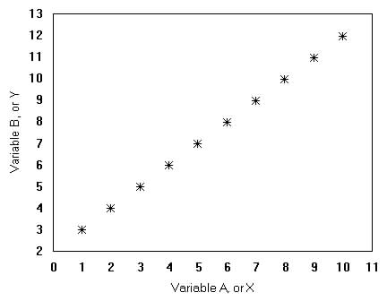
The number statistics used to describe linear relationships between two variables is called the correlation coefficient, r.

Correlation is measured on a scale of -1 to +1, where 0 indicates no correlation (Figure 3.2c) and either -1 or +1 suggest 
high correlation. Both -1 and +1 are equally high degree of correlation.

High Correlation - if one variable can consistently predict the value of the other variable, then a high degree of correlation
exist between them. Figures 3.2a and 3.2b.

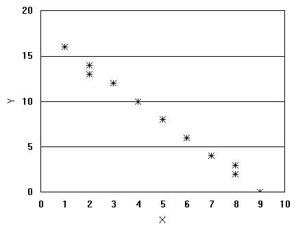
When two variables correlate and when the value of one increases as the value of the other decreases we say the
relationship between both variables shows a negative correlation.

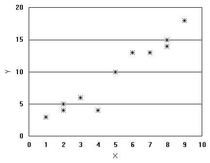
Moderate correlation is often suggested by a correlation coefficient of about 0.7. There is no absolute number guide for
correlation coefficient that tell when a two variables have low to high degree of correlation; however, r closed to -1 or +1 
suggest a high degree of correlation, values closed to 0 suggests no correlation or low correlation and values 
between 0.7 and 0.8 are moderate see Figure 3d.

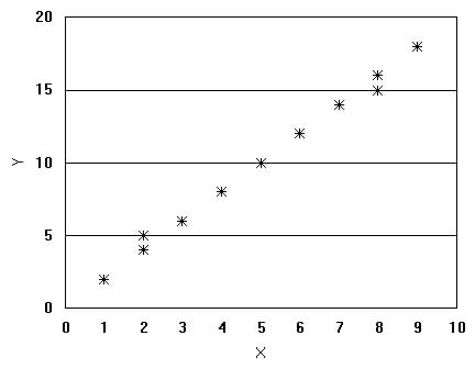
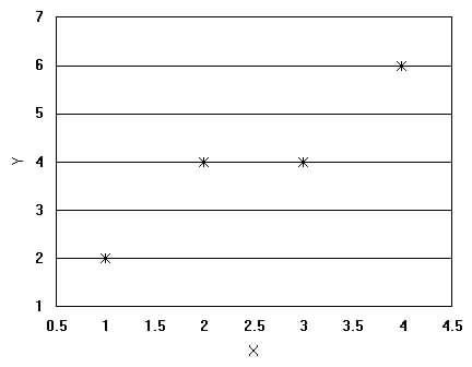
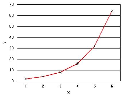
A graph of the data may also show the degree of correlation between variables, see Figure 3.2 below.

Figure 3.2 Graphs of Correlation Plots
 

(a) Positive, High Correlation close to +1	(b) Negative, High Correlation close to -1
(c) No Correlation, r = 0	(d) Moderate correlation, r about 0.7

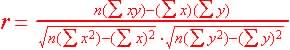
3. Know how to calculate the correlation coefficient, r from a set of paired data.

The correlation coefficient, r show the degree of linear relationship between two variables. So given pairs of values 
for variables X and Y, designated (x, y), r is given by the following formula:

where s_x and s_y are the standard deviations for x and y variables respectively.

is the sum of all values or function of values. A better formula to compute the linear correlation coefficient, r is:

Correlation coefficient, r computational formula:

Example: Compute the correlation coefficient for the pairs of values for the two variables below:
 

Tables of values: Table 3.1     x y 1 2 2 4 3 4 4 6	Summation Table:Table 3.2     x y xy x2 y2 1 2 2 1 4 2 4 8 4 16 3 4 12 9 16 4 6 24 16 36
Correlation coefficient statistics, r So r = 0.95	Scattered Plot of Data:

Workshop 3a. Correlation Example: Calculate the Correlation Coefficient of the following pairs of data:
 

Table 3.3 Correlation Coefficient Computational Matrix -  Correlation Coefficient Program

x y xy x2 y2 10 12       15 9       20 7       25 6       30 4       (a) Compute r from formula:  (b) Draw a scattered plot of the data and (c) State the degree of correlation between the variables. (d) Compare results to General Statistics (Simple Linear Regression, r from r2 ) http://www.compute.uwlax.edu/stats/

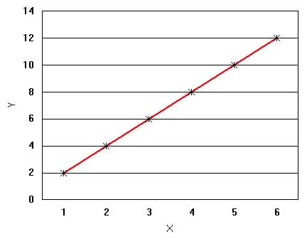
4. Know the meaning of linear and nonlinear relationships and the relevance of each to correlation analysis.

A linear relationship is one where a change in value of one variable will have a consistent change in value of the 
other variable at all values of the variables. Also if a non horizontal straight line can connect the pair of points of
both variable approximately then the relationship is linear, see 

Figure 3.3a.

A nonlinear relationship exist when the pairs of points of both variables cannot be connected or approximated by 
a straight line or change in values of one variable cause the change in value of the other variable to change 
by different amount, see Figure 3.3b.

Figure 3.3 Linear and Nonlinear Relationships
 

(a) Example of a Linear Relationship

(b) Example of a Nonlinear Relationship

5. Know the effect of changing units of X and / or Y on the correlation coefficient.

Adding, subtracting, multiplying or dividing a constant to all of the numbers in one or both variables do not change
the correlation coefficient.

6. Know the types of scale required for correlation analysis.

Correlation analysis requires that both variables be measured at least at the level. Simply for each values of X, Y is
measured and results paired: (x, y)

7. Know the effect of the unreliability of the variables on the correlation coefficient.

If values of either variable are unreliable (that is, they have measurement or other errors) then the correlation coefficient
will be lower than what is expected (underestimate the relationship between the variables).

8. Know the effect of restricted or truncated range on the correlation coefficient.

If either of the variables has a restricted range (not the full range of values of the population of interest) then the 
correlation coefficient will be low.

9. Know the relationship between correlation and causation.

High correlation between variables does not mean that one variable cause the other.

High correlation just suggest that a causal relationship might exist.

No correlation assume no causal relationship exists between two variables; however, lack of correlation may be due
to other factors such as, poor measurements, restricted range, non-linear relationships or other extraneous factors 
that mask the true relationship.

10. Know how to interpret a correlation coefficient, r in terms of (coefficient of determination) 
percent of variance, r².

The coefficient of determination, r² is the square of the correlation coefficient, r

The coefficient of determination is equal to the percent of variation in one variable that is accounted for (predicted) 
by the other variable.

Though the correlation coefficient is useful to determine the degree of linear relationship between tow variables, 
the coefficient of determination allows us to interpret the relationships in terms of variations, a more familiar term.

=Proportion of variation in y values that is explained by the linear relationship with x.

The greater the proportion of explained variation, the closer are the y values and y values, hence the stronger the
linear relationship. 

The simplest way to calculate the proportion of explained variation over the total variation (coefficient of determination, r²) 
is to compute r and square it.

Linear  regression is a methodology used to find a formula that can be used to relate two variables that are linearly related,
i.e. given the value of one variable or attribute, one may find the corresponding value for the other variable or attribute. 
There should first be a meaningful relationship between both variables before the linear regression formula is determined. 
The process of finding a formula is called regression. A regression  formula may also be found to relate more than two variables,
but only the method of relating two variables will be discussed in this course.

The regression formula found looks something like this:  y=mx+b,  where m and b are constants determined by the regression
procedure and y and x are the variables being related.

1. Know the difference between correlation and regression analyses.

Correlation analysis is concern with knowing whether there is a relationship between variables.

Regression analysis is concern with finding a formula that represents the relationship between variables so as to find an
approximate value of one variable from the value of the other(s)

2. Know how to interpret the equation of a linear regression formula, y=mx+b.

A linear formula when graphed produced a straight line and is represented by the formula y=mx+b for variable X and Y.

This linear formula is also called the regression line.

The regression formula is used to predict values of one variable, given values of another variable. Prediction can be made 
from X to Y or from Y to X although usually X is used to predict Y (where X is the input variable and Y is the output variable).

The slope of a linear line is represented by the value of m in the regression formula above, and it is the rate of change of Y
relative to change in X, this number is a constant value for linear regression formulas. The slope is sometime called the 
regression coefficient . When the slope is positive, the line is an increasing function, that is, as x increases in value the 
value of y also increases: this in known as positive linear relationship (see Figure 3.3a). When the slope is negative, 
the line is a decreasing function, that is, as x increases in value the value of y decreases: this is known as negative linear 
relationship (see Figure 3.2b).

If X and Y are plotted on a graph and the relationship is approximately linear, a regression line or equation may be used 
to approximate the relationship between the variables, this regression line is useful when it is associated with a 
high degree of correlation and a low standard error of estimate.

The point where the regression line crosses the Y axis is called the y-intercept and is represented by b in the regression formula. 
The y-intercept, b is also the value of the Y variable when the X the value of the X variable is equal 0.

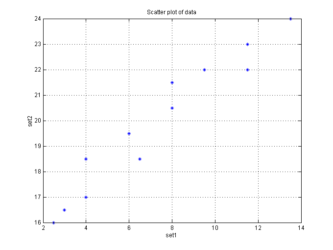
Figure 3.4 below shows a regression line with data scattered about the line (an estimate), where b=x, the slope, m = y.

Example find the regression equation for the data in Table 3.4 below using the online statistics tool 
(Simple Linear Regression plot)
 

Table 3.4 Salary Data of 12 workers     Years of Service Salary, $1000 6 19.5 8 20.5 3 16.5 11.5 22 13.5 24 4 17 2.5 16 9.5 22 11.5 23 6.5 18.5 8 21.5 4 18.5

Figure 3.4 Scattered Plot of Data

The regression formula is y = 14.7345 + 0.70666x, where 14.7345 is the y-intercept and 0.7067 is the slope.

3. Know the meaning of residual.

The predicted value is the value of the Y variable that is calculated from the regression line. 
The predicted value is often designated by , called y-hat.

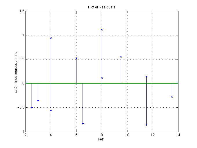
The residual is the difference of the actual value from the predicted value:
 

Residual = Actual - Predicted

Example (Using pervious example above)
 

Table 3.4 Salary Data of 12 workers     Years of Service, x Actual value, y (A) Predicted value (P) y = 14.73 + 0.71x Residual, (A)-(P) 6 19.5 18.99 0.51 8 20.5 20.41 0.09 3 16.5 16.86 -0.36 11.5 22 22.78 -0.78 13.5 24 24.32 -0.32 4 17 17.57 -0.57 2.5 16 19.17 -3.17 9.5 22 21.48 0.52 11.5 23 22.9 0.1 6.5 18.5 19.35 -0.85 8 21.5 20.41 1.09 4 18.5 17.57 0.93

Figure 3.5 Plot of Regression Line and Residual (The difference between the actual values above and below the regression line - 0)

Residual is the same as the error of estimate, e, where e = y - 

Example when x = 6.5 above, y = 18.5 and the predicted value,  = 19.35, 

e = 18.5 - 19.35 - -0.85

4. Know how to determine linear relationship from a scattered plot.

If the points in a scattered plot cluster about a non-horizontal line (horizontal line has a zero slope),
then the relationship between the x and y variable is approximately linear (see Figure 3.5. 

above).

5. Know the meaning of the Least Square Criterion.
 

The Least Square Criterion is a criterion to find the best fit of a regression line to the scattered plot of the data. If we define the sum of squares for error, SSE to be the sum of squares of the error terms: For Example above SSE for residual is 4.9252

The line of best fit or regression line is the line that best fits the data is the line in which the sum of squares for error, 
SSE, is minimum. 

6. Know the criteria used for forming the regression equation.

The regression equation or formula meets the "least Square" criterion - the sum of square of the residual is at its minimum.

7. Know how to predict using the correlation coefficient and z-scores.

A predicted z-score (for the Y variable) is equal to the correlation coefficient, r times the corresponding z-score for X.

Example, if the z-score for a value of the X variable is -1.12 and the correlation coefficient is 0.77, then the z-score for
the corresponding Y value is -1.12 x 0.77 = -0.86

Given (x, y): then z-score(y) = z-score(x) times correlation coefficient.

8. Know how to calculate the regression equation for a set of data using Least Square or best fit formulas:

To find the parameters for a linear regression formula, y=mx+b.
 

For the linear regression formula , the best fit line: , where  is the average for all y values and  is the average for all x values.

Example Shows how this is done for a set of data:

Table 3.5 Best fit calculation of regression line
 

x	y	xy	x2
6	19.5	117	36
8	20.5	164	64
3	16.5	49.5	9
11.5	22	253	132.25
13.5	24	324	182.25
4	17	68	16
2.5	16	40	6.25
9.5	22	209	90.25
11.5	23	264.5	132.25
6.5	18.5	120.25	42.25
8	21.5	172	64
4	18.5	74	16
=7744

There the slope is 

And 

So y=0.71x+14.71

Workshop 3b - Regression Example  Using Least Square Formulas find the best fit for the following data:
 

Linear Regression Program x y xy x2 16 18     18 21     13 12     11 9     13 11     14 17     12 13     19 22     11 8     16 19     18 22     14 14

Slope

Write Regression Equation:

9. Know appropriate steps to take before computing a regression equation (line).

Do not blindly compute the regression line, look first at scatterplot, and investigate linearity with statistics 
such as correlation coefficient.

(a) Study Scattered plots (check for linearity)

(b) Examine correlation coefficient or better yet the coefficient o f determination

10. Know the relationship of outliers or unusual observation on regression line.

Unusual observations are point that seem to deviate for the clusting of the other points.

An outliers is an observation that substantially affect or alter the regression line.

When an unusual observation have a large influence on the regression line it is called an influential observation.

Influential unusual observations that are identified as outliers are not included in calculating the regression line.
 

The coefficient of determination, r² is another way of looking at the correlation coefficient, r, it is the square of the
correlation coefficient or better yet the correlation coefficient is the square root of the coefficient of determination. 
Since variations and deviations are easily interpreted quantities, the coefficient of determination attempts to look at strength 
of relationships in terms of deviations from some expected or defined set of values (the regression line or best-fit line).

11. Know the meaning of total variation, unexplained variation, and explained variation.

Given a set of data, its scatterplot and regression line,

Total deviation (or variation) is the sum of the squared deviation of each value from the mean of that variable. For the variable,
Y it is the variation that exists within the distribution of the Y variable before prediction, see Table 3.6. 
So the total sum of square deviation is :

Total deviation = Explained deviation + Unexplained deviation
 

for individual value of y. for all values of y or the sum of square deviation.

Explained deviation or variation is the sum of squared deviations of each predicted value from the variable's mean:
the average sum of square explained deviation is :

Unexplained deviation or variance is the sum of the squared deviations of each value of the variable from its predicted value,
so the sum of square unexplained deviation is :

Table 3.6 Variation table (From Table 3.4)
 

Actual value, y ()	Predicted value ()	Deviation deviation ()2	Explained deviation ()2	Unexplained deviation or error or residual (  )2
19.5	18.99	0.7136	0.8587	0.2601
20.5	20.41	0.3403	0.2434	0.0081
16.5	16.86	11.6736	9.3432	0.1296
22	22.78	4.3403	8.1987	0.6084
24	24.32	16.6736	19.3893	0.1024
17	17.57	8.5069	5.5068	0.3249
16	19.17	15.3403	0.5575	10.0489
22	21.48	4.3403	2.444	0.2704
23	22.9	9.5069	9.9003	0.01
18.5	19.35	2.0069	0.3211	0.7225
21.5	20.41	2.5069	0.2434	1.1881
18.5	17.57	2.0069	5.5068	0.8649
Mean is n=12		Total deviation :	:	:

12. Know how the coefficient of determination, r² can be computed from the total deviation or variation
and the explained deviation

The coefficient of determination, r², is the ratio of the explained deviation over the total deviation.
 

, Where n cancels out.

Example; From Example in Table 3.6 

, so r=0.90 (to be verified)

13. Know the meaning of how to interpret the standard error of estimate.

The standard error of estimate,  is the standard deviation of the residuals, if the residual is e, then
the standard error of the estimate is:

The standard error of the estimate is an indication of the accuracy of the prediction or regression equation.

If there is perfect prediction, the sum of residuals will be equal to 0 (similar to Figure 3.3a).

If there is no prediction the standard error of the estimate will be the same as the standard deviation of Y.

Residuals are assumed to be normally distributed for random collection of data. So a plot of the residual should
look like a normal distribution or bell curve plot.

The best fit or least square line attempt to fit a linear line to the scattered plot of the data so as to minimize
the sum of square of the residuals or the standard error of estimate.

14. Know common mistakes to avoid when using correlation and regression analyses.

Avoid equating correlation with causality. Strong correlation between variables does not mean that one cause the other.

Avoid unwarranted extrapolation of inferring or making predictions outside of the range of values of the variables studied.

Example: If your study focused on students age 13 to 16, it might be questionable using such results to 
extrapolate for age 21.