A class of continuous random variable is that of the normal random variable. Most researcher make assumptions based on the normal distribution of this variable because it offers many useful generalizations and rules or theorems, such as the Central Limit Theorem.

The probability distribution or density function of a continuous random variable is related to the area under the curve of the function and not the relative frequencies as do discrete random variables.

1. Know how to construct a probability distribution or adjusted histogram from a frequency distribution table of a continuous random variable.

The conversion of a frequency distribution to a probability distribution is also called an adjusted histogram. This is true for continuous random variables.

To convert a frequency distribution to a probability distribution, divide area of the bar or interval of x by the total area of all the Bars.

A simpler formula is:

, N is the total Frequency and w is the interval of x.

Example (From a frequency distribution table construct a probability plot).
 

Table 6a.1. Frequency Table:     x Frequency, f 10 30 15 60 20 80 25 50 30 30 35 20 40 10 45 5 The width of each bar or interval, w = 5(20-15, or 45-20, etc.)  See Example below for Area	Table 6a.2. Adjusted Histogram - Probability Distribution, w = 5     x Frequency,  f f/(Nw) 10 30 0.0211 15 60 0.0421 20 80 0.0561 25 50 0.0351 30 30 0.0211 35 20 0.014 40 10 0.007 45 5 0.0035   N=285
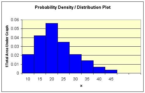
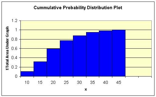
Figure 6a.1. Probability Distribution Plot.	Figure 6a.2. Cumulative Probability Distribution Plot

2. Know how to interpret the graph of a continuous probability distribution or adjusted histogram.

The graph of a probability distribution in addition to telling us about the nature of the random variable can give us information about the following:

(1) The probability density of the variable

(2) The probability of x at any point

(3) The probability between an interval a and b

(4) The cumulative probabilities

(5) The probabilities, at certain range of values.
 

Knowing how to read or determine these information is important for the rest of this course, since the uncertainty or probability of various distributions will be needed to make inference or judgment about sample data or statistics.

Example: Consider the probability distribution plot of a continuous random variable shown in Figure 6a.3 below:
 

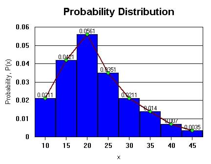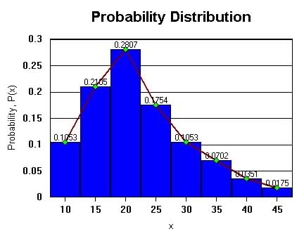
Figure 6a.3. Probability Distribution Plot of Continuous Random variable, x P(x between 17.5 and 22.5)=0.0561 x 5 = 2805 (Area between the interval) Area = interval width x average height

The Nature of the random variable.

The probability distribution plot, gives and indication of the shape of the variable x. 

If the random variable is continuous a histogram is just a rough depiction of the variable distribution since the histogram shows only discrete values of the variable. If the frequencies were collected for more data points within the interval of the continuous scale and a curved line is drawn connecting the points as shown in Figure 6a.3 above we call this graph a continuous curve.

P(x) can be viewed as f(x), a function or model that represents the probability of x, P(x) at different values of x.

In more advanced mathematics (beyond the scope of this course), statisticians may by observation and modeling of the shape of the probability curve or distribution or probability density function determine appropriate mathematical formulas for each P(x).

This modeling is called a function, and is often given the equation y =f(x), when y is the dependent variable recorded on the vertical scale which is related to the P(x). The independent variable is x.

Note: In textbooks most continuous variable functions are indicated by curve line graphs, but in actual data collection and summaries, the adjusted histogram is use as an approximation.

(1) The probability density of the variable

From the probability plot the individual probability values at various values of x can be determined or approximated.
 

The probability that a continuous random variable assumes some value in an interval is represented by the area under the portion of the continuous curve of that interval. Prob[Interval of x] = Area of Probability Destiny Function for that same interval

Table 6a.3. Probability - Area under Graph The interval width, w = 5 (intervals do not overlap)     x Interval P(x) Area= wP(x) 10 7.5 to 12.5 0.0211 0.1053 15 12.5 to 17.5 0.0421 0.2105 20 17.5 to 22.5 0.0561 0.2807 25 22.5 to 27.5 0.0351 0.1754 30 27.5 to 32.5 0.0211 0.1053 35 32.5 to 37.5 0.014 0.0702 40 37.5 to 42.5 0.007 0.0351 45 42.5 to 47.5 0.0035 0.0175       Sum = 1

 

The total area under the probability plot add up to 1.

Problems: (assume for problem above that the intervals do not include the upper bound, i.e. An interval of 7.5 to 12.5 does not include the value 12.5)

1. Find Pr[ x < 22.5]

P(x< 22.50 = P( ) = Area under the graph from 7.5 to 22.5 

From table above P(x < 22.5) = 0.1053 + 0.2105) = 0.3158

2. Find the Pr[ 17.5 < x < 32.5] = Area of [ 17.5 < x < 32.5] 

= 0.2807 + 0.1754 +0.1053 = 0.5614

(2) The probability of x at any point

For continuous random variable the probability for an exact value of x is = 0, since the interval width is so small that is almost impossible to tell the exactly value of P[x=a], where a is an exact value or number.

(3) The probability between an interval a and b

1. Find Pr[ x < 22.5]

P(x< 22.50 = P( ) = Area under the graph from 7.5 to 22.5 

From table above P(x < 22.5) = 0.1053 + 0.2105) = 0.3158

2. Find the Pr[ 17.5 < x < 32.5] = Area of [ 17.5 < x < 32.5] 

= 0.2807 + 0.1754 +0.1053 = 0.5614

(4) The cumulative probabilities

The Cumulative probability is the probability of the variable up to a certain value a.

Example. Find Pr[ x < 22.5]

P(x< 22.50 = P( ) = Area under the graph from 7.5 to 22.5 

From table above P(x < 22.5) = 0.1053 + 0.2105) = 0.3158

(5) The probabilities, at certain range of values.
 

For a continuous random variable, x Pr[) is the same as Pr[a < x < b]

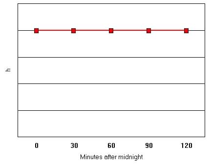
Problem: Assume that the time of birth of a New Year's baby at a city hospital will be some random time between midnight and 2:00 am. Let x be the number of minutes after midnight that the baby will be born. So . (60 minutes in a hour - 2 hours after midnight gives us 120 minutes). The graph of the probability distribution is shown below (x is a uniform distribution - same value at each value of x).
 

Uniform Distribution of x (continuous random variable).

(a) What is the area of under the graph? What is the height of h? (b) What is the probability that the New Year's baby will be born (i) Before 12:30 am? (ii) After 1:15 am? (iii) Between 12:45 and 1:00 am? (iv) Before 12:15 am or after 1:30 am? (c) Express parts (i), (ii), and (iii) of part (b) in one of the following forms: P(a<x<b), P(x<a), or P(x>a)

Worksheet Adjusted Histogram for Probability Distributions of Continuous Random Variables.

To calculate the Probability Distribution for a Continuous Random Variable

Probability - Area under Graph - Example

The interval width, (1) w = ____ (intervals do not overlap)
 

Midpoint Values x	Interval Values	P(x)	Area= wP(x)
			Sum = 1