Many random variables exhibits the properties of a normal distribution, appears symmetrical or bell shape. The normal distribution is a well known distribution whose probability distribution or values at any point or interval is well known.

1. Know the properties of the normal distribution.
 

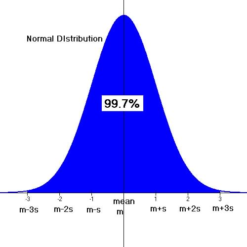
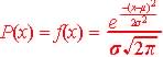
Properties of Normal Distributions.1. The graph of the normal distribution assumes a symmetrical distribution or bell-curve. The mean is the central point of the normal distribution. At the mean the distribution is symmetrical or have a mirror image about this point. 2. The mean , median and mode of the normal distribution have the same value. 3. Though not required for this course, the formula for the probability distribution of the normal distribution given by the formula:, where  can be estimated by the sample mean and  by the sample standard deviation.

Figure 6b.1 Show a graph of the normal distribution.
 

2. Know the properties of the standard normal distribution.
 

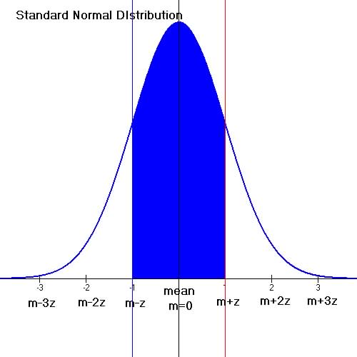
The standard normal random variable is a normal variable with mean = 0 and standard deviation = 1. Its value is represented by the symbol, z. and  All normal random variables can be converted to the standard normal variable, z.

Figure 6b.2 Graph of the standard normal distribution.
 

3. Know how to interpret the probability under the curve for the standard normal distribution.

At any z value of the standard normal probability distribution the reference table gives the cumulative probability (area under the curve) up to that value.

Example, the probability of z = -3.01 from the table is 0.000967671.

The extreme values of z are , z can be a very large negative number of a very large positive number, In practice rarely does one exceed z = -6 negatively or z = +6 positively.

For most normal random variables 99.9% of the population or distribution is within a z value of .

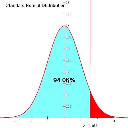
Example: Find the probability of z < 1.56.
 

From the reference table, the area under the standard normal distribution, i.e. the probability for z = 1.56 is 0.94062005 or 94.06% of the area is z < 1.56.

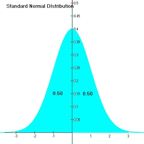
3. Know how to use the symmetry of the standard normal distribution the find probability of range of z values.

Because the standard normal distribution is symmetrical about the mean or center, the area under the curve or probability on either sides of the mean or center line is each equal to 0.50 or 50%.
 

Figure 6b.3 Symmetry of the Standard Normal Distribution

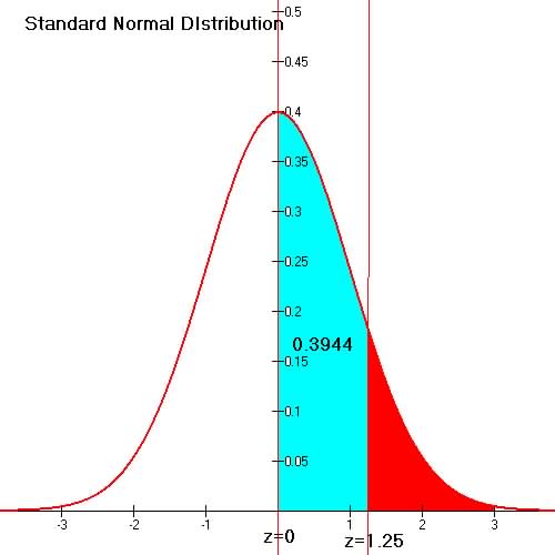
Example: Find the probability of the normal variable z, for 0 < z < 1.25.

That is , find Pr[0 < z , 1.25].

Two ways to do this (1) Pr[z=1.25] - 0.50 = 0.89435016 - 0.5 = 0.39435016 or 0.3944 or

(2) Pr[z=1.25] - Pr[z=0] = 0.89435016 - 0.5 = 0.3944
 

Example: A company makes widgets and the flatness of widgets are supposed to be 0 mm (its mean), if the standard deviation is 1 mm, what is the probability that flatness will be between -1.45 and +1.50?

Assume that flatness is a standard normal distributed random variable and that negative flatness means surface curves downwards and positive flatness means it curves upwards).

This is a standard normal distribution since its typical or average value or mean is 0 and its standard deviation is 1.

So the Probability that flatness, z is -1.45 < z < 1.50 can be determined using values from the standard normal reference table.
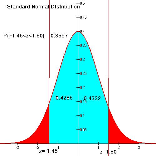
  Probability is the Area between z = -1.45 and 1.50.

P[-1.45 < z < 1.50] = Pr[z = or <1.50] - Pr[z = or < -1.45] = 0.9332 - 0.0735 = 0.8597 or

Note: Pr[z = 0] = 0.50

P[-1.45 < z < 1.50] = Pr[-1.45 < z < 0] + Pr[0 < z < 1.50] =

= (0.50 - 0.0735) + (0.9332 - 0.50) =0.4265 + 0.4332 = 0.8597.
 

Note: When working out probability for normal distribution it is a good practice to sketch the values for z or x and indicate the probability and add or subtract values for probability depending on interval of z of interest.

Example above illustrated by sketch below:P[-1.45 < z < 1.50] = 0.8597
 

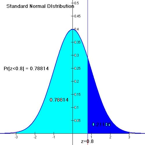
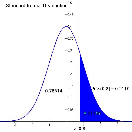
Example: Find the probability of z > 0.8.

A sketch of the interval of interest shows that since the total probability or area under the curve is 1.0 and Pr[z = 0.8] = 0.78814,

Then Pr[z=0.8] = 1 - Pr[z=0.8] = 1 - 0.78814 = 0.21186.
 

Pr[z=0.8] is Area up to z = 0.8

Pr[z> 0.8] is Area after z= 0.8

4. Know how to find the z value for a given probability.

By convention or notation the probability of a given z value at a point a is referred to as the P[z> a].

This notation is represented symbolically by the notation z_a or , where a or alpha is called the significant level.

The find the probability of a given value of z, locate the associated probability from the reference table.
 

Lookup the corresponding value of z associated with the probability 1- a or  in the reference table. Find values of z for  = value of z such that the area under the curve of the standard normal distribution to the right of it is 0.10, this is the same as finding z value corresponding to a probability of 1 - 0.10 = 0.90, i.e. the z value that gives Pr[z] > 0.90.

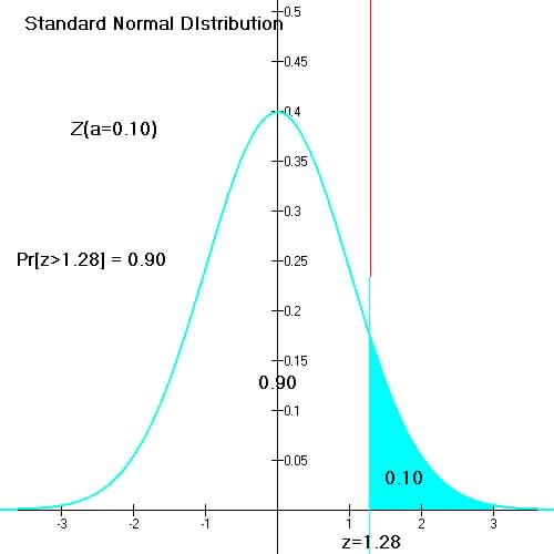
For example, to find Pr[z>a]=0.95 or z_0.95 look up 1- 0.95 = 0.05 in the reference table and the corresponding z value associated with it is -1.65. Here are a few more illustrated examples of z_a :

Find values of z for  -  Lookup z value for P[z]= 1-0.10 =0.90 (reference table) = 1.28

Find values of z for  - Lookup z value for P[z] = 1-0.05=0.95  = 1.65 Find values of z for  - Lookup z value for P[z] = 1-0.90=0.10   = -1.28 Find values of z for  - Lookup z value for P[z] = 1-0.80=0.20   = -0.84 Find values of z for  - Lookup z value for P[z] = 1-0.025=0.975   = 1.96 Find values of z for  - Lookup z value for P[z] = 1-0.975=0.025   = -1.96

Workshop Problem - Use the standard normal reference table to find the following, values of z or its corresponding probabilities: (assume z is a standard normal variable with mean = 0 and standard deviation = 1).

(a) Pr[z , 1.43]

(b) Pr[0 < z < 1.51]

(c) Pr[-2.01 < z < 1.84]

(d) Pr[z < ______] = 0.9575

(e) Pr[z > ______] = 0.105