Tony

Yen and the art of learning statistics without really trying Am I Normal?

Rose

Programs Normal Distributions.

During a study session at James White's Library, one hour before closing.

Tony: "Rose, am I normal?"

Rose: (silence)

Tony: "I meant statistically, what is normal and how can I determine if something is normal or not?"

Rose: "To answer your question, we must first have some idea of what is normal or a standard or reference to compare things to."

"Could I say that a 50-pounds new born baby is normal or that a 1-pound new born is normal?"

"Could I say that a vehicle with 4 wheels is normal or typical?"

"To answer these question or any question about what is or isn't normal we must have some idea of possible values of normality."

"So when you ask me 'are you normal?', are you asking me: do you have a normal height (or other characteristics) or are you crazy?"

"The answer to are you crazy is not for a statistician to decide, but if you have the time, I will give you my opinion."

Tony: Ignoring Rose: "Statistically how do we determine normality?"

Rose: "It appears that every event or statistics or parameter or characteristic seems to have some typical value."

"According to the Central Limit Theorem, if we conduct a study with a large enough sample size (usually sample size greater than or equal to 30), we would observed that the characteristics or random variable that we are studying would give us a typical or normal value with some degree of certainty." "Furthermore, if we continue to take many such samples, the means of these samples will form a normal distribution or a distrubution that is symmetrical about the true mean of the population mean we are trying to estimate."

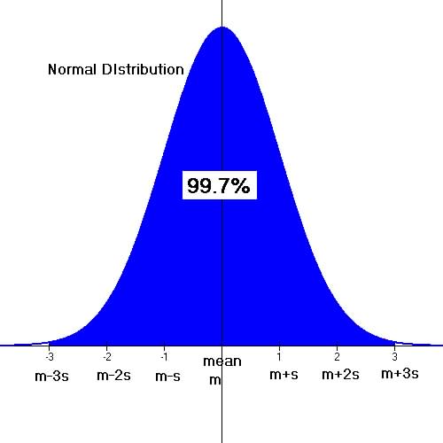
"Visually, if your were to draw a frequency histogram of the data it would look like a bell shape curve or a normal distribution curve."

"What the Central Limit Theorem says in effect is that all random variable have a typical value at which if enough data is collected or experiments are conducted, the data would tend to cluster symmetrically about this typical value; for example, if we which to determine what score students tend to get on the SAT verbal section we should find a bell shape distribution of scores clustered around maybe a typical score between 500 and 600."

Graph of a bell shape or normal distribution

"With discrete random variable the probability distribution is calculated using the values of the variable and the relative frequencies of this distribution, but with continuous random variable we need to access probability differently since the values of each variable is not a specific or discrete value."

"Probability distribution for a continuous random variable is related to the area under the frequency distribution for various intervals of the random variable".

Tony: "Hmmm?"

Rose: ", that is the area of an interval for a chunk of an histogram would give you the probability for interval."

note: the area of an interval of x is the height of the graph divided by the width of the interval and the P[interval of x] = Area of interval divided by the total area under the graph. When I was in college we used to cut out the area of the curve from cardboard and weight it , then cut out the protion of the interval of interest and weight, then find the probability using the ratio of the two weights.

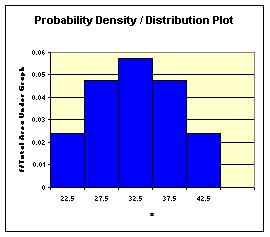
"What if you had the following information about a continuous random variable x, with associated frequencies for a fixed ranges of values for x:"
 

Range of values for x	Interval Mid Point	Frequency
20-25	22.5	5
25-30	27.5	10
30-35	32.5	12
35-40	37.5	10
40-45	42.5	5

"A probability density function would be determine using the Probability Density of Continuous Program to get the following:"
 

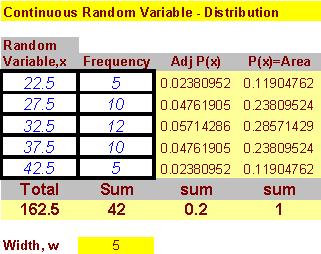"Example, Pr[x=32.5] = 0.2857"

"When a continuous random variable looks like a normal distribution or bell shape curve we now have a normal random variable."

"And because the properties of the normal distribution is well known, we can make very meaningful inference about the information or statistics
found from the probability distribution of that variable."

Tony: "So once we have assumed that a random variable is normal, where do we go from there?"

Rose: "The standard normal distribution is a powerful application of statistics that allows you to simplify the calculation or assessment of any random variable or characteristics that we consider normal and its states simply:

The central point or middle of the normal distribution can be considered as a reference point with a value of 0 and all other points are compared to this central 0 point by its number of standard deviations from 0; one standard deviation is given a value of 1."

"For example, if we have a set of data from a normal distribution with a central point or mean of 400 and a standard deviation of 100, then a sample data point of 600 is:

Let the mean of 400 be a reference point of 0 so 600 differs from 400 by 200 or + 2 standard deviation about the mean." That is, mean + 2 x standard deviation = 600 = 400 + 2(100).

"Later this concept is used to develop a statistics called the z-score, which is the number of standard deviations of the data about the mean (this comes from the standard normal distribution concept.)"

Given any normal variable, x with mean =  and standard deviation =  , we define the z-score or standard score
(the z value of the standard normal distribution) has:

Example: Find the z-score or z value of a normal variable whose value is 45 if its mean is 50 and standard deviation is 5.

The value of the random variable is x = 45, and  ,

, which means that x = 45 is 1 standard deviation below the mean since the z-value is negative 1.

Example: Find the z-score or z value of a normal variable whose value is 650 if its mean is 500 and standard deviation is 100.

The value of the random variable is x = 650,   and  ,

, which means that x = 650 is 1 ½ standard deviations above the mean since the z-value is positive.

So z = 1.5.

Tony: "I once read that in many discussions or problems involving the normal random variable rarely do we find its mean to be equal to 0 or its standard deviation to be equal to 1".

Rose: "That is true, that is why given a random variable which is normal, one tries to determine its z-score value from the formula above and then look up its probability from a standard normal probability reference table; the z-score is listed on the left and the probability values within the table."

Example if we get  z=1.96, the probability of that value is Pr[z=1.96] = 0.975

See more examples of z-score calculations:

Tony: "Could you explain a little bit more about the Central Limit Theorem you mentioned it earlier, before the library closes?"

Rose: "In simple terms, when a sample gets large (sample size n) the sample frequency polygon will start to look like a normal distribution with mean same as you would calculate the mean of a normal distribution but its standard deviation or standard error of  is ."
 

Central Limit Theorem: As samples size increases the sample distribution approaches the normal distribution.

Example: If you sample 40 college students to determine their height, then the mean height would be the sum of all the heights divided by 36 and the standard error would be the standard deviation divided by the square root of 36, the sample size.
 

For sample hypothesis testing or inference about the population from sample data we use the  standard error instead of the standard deviation.

Tony: "Well as Forest Gump's mother  would have said: 'Normal is as normal looks' ."

Rose: "Who is Forest Gump?"

Tony: "You are definitely not normal, I got to go, I am meeting Obi Wan for dinner!"

Rose: (profound silence)